How To Interpret Partial Eta Squared Effect Size

Outcome size is an interpretable number that quantifies
the divergence between information and some hypothesis.

Overview Effect Size Measures
Chi-Square Tests
T-Tests
Pearson Correlations
ANOVA
Linear Regression

Statistical significance is roughly the probability of finding your data if some hypothesis is true. If this probability is low, so this hypothesis probably wasn't true after all. This may be a nice first footstep, only what nosotros really need to know is how much practise the data differ from the hypothesis? An effect size measure summarizes the answer in a single, interpretable number. This is important considering

issue sizes permit us to compare furnishings -both inside and beyond studies;
we need an effect size measure to estimate (1 - β) or power. This is the probability of rejecting some null hypothesis given some alternative hypothesis;
fifty-fifty earlier collecting whatsoever information, effect sizes tell us which sample sizes we need to obtain a given level of ability -often 0.80.

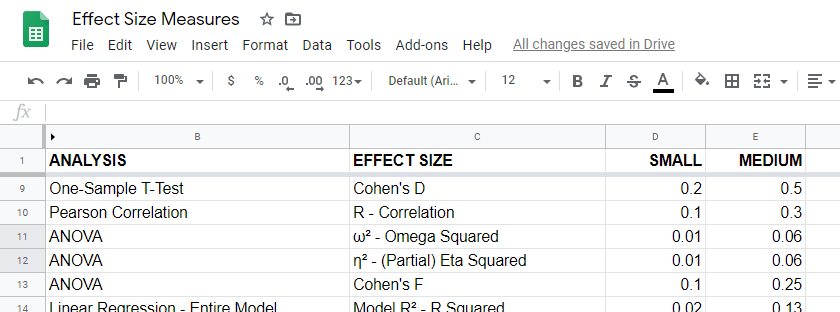
Overview Issue Size Measures

For an overview of effect size measures, delight consult this Googlesheet shown below. This Googlesheet is read-only merely tin can be downloaded and shared as Excel for sorting, filtering and editing.

Chi-Square Tests

Common effect size measures for chi-square tests are

Cohen's W (both chi-square tests);
Cramér'due south 5 (chi-foursquare independence test) and
the contingency coefficient (chi-foursquare independence test) .

Chi-Foursquare Tests - Cohen's W

Cohen'south W is the effect size measure of choice for

the chi-square independence exam and
the chi-foursquare goodness-of-fit examination.

Basic rules of thumb for Cohen's Westward⁸ are

pocket-size result: w = 0.10;
medium effect: w = 0.30;
large issue: w = 0.50.

Cohen's West is computed every bit

$$W = \sqrt{\sum_{i = 1}^thou\frac{(P_{oi} - P_{ei})^2}{P_{ei}}}$$

where

$P_{oi}$ denotes observed proportions and
$P_{ei}$ denotes expected proportions nether the nil hypothesis for
$chiliad$ cells.

For contingency tables, Cohen's West can likewise exist computed from the contingency coefficient $C$ every bit

$$West = \sqrt{\frac{C^2}{1 - C^two}}$$

A third pick for contingency tables is to compute Cohen'south W from Cramér's V every bit

$$W = V \sqrt{d_{min} - 1}$$

where

$V$ denotes Cramér's Five and
$d_{min}$ denotes the smallest tabular array dimension -either the number of rows or columns.

Cohen'due south Due west is not available from any statistical packages we know. For contingency tables, we recommend computing information technology from the same contingency coefficient.

For chi-square goodness-of-fit tests for frequency distributions your best option is probably to compute it manually in some spreadsheet editor. An example calculation is presented in this Googlesheet.

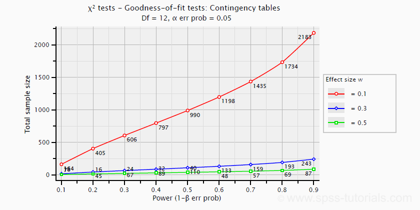
Ability and required sample sizes for chi-foursquare tests can't be straight computed from Cohen'due south W: they depend on the df -short for degrees of liberty- for the test. The instance chart below applies to a five · 4 table, hence df = (five - 1) · (four -ane) = 12.

T-Tests

Mutual consequence size measures for t-tests are

Cohen'due south D (all t-tests) and
the indicate-biserial correlation (just contained samples t-test).

T-Tests - Cohen's D

Cohen's D is the outcome size measure of option for all three t-tests:

the independent samples t-exam,
the paired samples t-exam and
the i sample t-test.

Basic rules of pollex are that^eight

|d| = 0.20 indicates a small effect;
|d| = 0.fifty indicates a medium outcome;
|d| = 0.80 indicates a large consequence.

For an independent-samples t-test, Cohen'southward D is computed equally

$$D = \frac{M_1 - M_2}{S_p}$$

where

$M_1$ and $M_2$ denote the sample ways for groups 1 and ii and
$S_p$ denotes the pooled estimated population standard deviation.

A paired-samples t-exam is technically a one-sample t-test on difference scores. For this examination, Cohen'due south D is computed as

$$D = \frac{M - \mu_0}{S}$$

where

$M$ denotes the sample mean,
$\mu_0$ denotes the hypothesized population mean (difference) and
$South$ denotes the estimated population standard departure.

Cohen's D is present in JASP but not SPSS. For a thorough tutorial, delight consult Cohen's D - Effect Size for T-Tests.

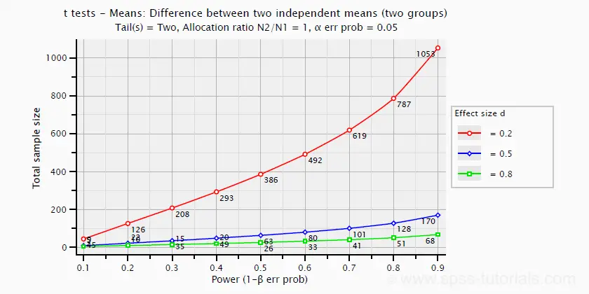
The chart beneath shows how power and required total sample size are related to Cohen's D. It applies to an independent-samples t-test where both sample sizes are equal.

Independent Samplest Test Sample Size Power Curve

Pearson Correlations

For a Pearson correlation, the correlation itself (often denoted as r) is interpretable as an effect size measure. Bones rules of thumb are that⁸

r = 0.10 indicates a pocket-size event;
r = 0.thirty indicates a medium effect;
r = 0.l indicates a big effect.

Pearson correlations are available from all statistical packages and spreadsheet editors including Excel and Google sheets.

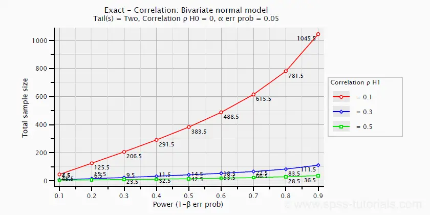
The nautical chart beneath -created in G*Power- shows how required sample size and ability are related to outcome size.

ANOVA

Common effect size measures for ANOVA are

$\color{#0a93cd}{\eta^two}$ or (partial) eta squared;
Cohen's F;
$\colour{#0a93cd}{\omega^2}$ or omega-squared.

ANOVA - (Partial) Eta Squared

Partial eta squared -denoted as η ²- is the effect size of choice for

ANOVA (betwixt-subjects, one-way or factorial);
repeated measures ANOVA (one-way or factorial);
mixed ANOVA.

Basic rules of pollex are that

η ² = 0.01 indicates a small outcome;
η ² = 0.06 indicates a medium effect;
η ^two = 0.14 indicates a large result.

Fractional eta squared is calculated as

$$\eta^2_p = \frac{SS_{effect}}{SS_{effect} + SS_{error}}$$

where

$\eta^2_p$ denotes fractional eta-squared and
$SS$ denotes effect and error sums of squares.

This formula also applies to one-manner ANOVA, in which case partial eta squared is equal to eta squared.

Fractional eta squared is available in all statistical packages nosotros know, including JASP and SPSS. For the latter, encounter How to Get (Fractional) Eta Squared from SPSS?

ANOVA - Cohen'south F

Cohen's f is an event size measure out for

ANOVA (between-subjects, one-way or factorial);
repeated measures ANOVA (one-manner or factorial);
mixed ANOVA.

Cohen's f is computed as

$$f = \sqrt{\frac{\eta^2_p}{1 - \eta^2_p}}$$

where $\eta^2_p$ denotes (partial) eta-squared.

Bones rules of pollex for Cohen'south f are that^viii

f = 0.10 indicates a small upshot;
f = 0.25 indicates a medium effect;
f = 0.xl indicates a large effect.

G*Power computes Cohen's f from various other measures. We're non aware of any other software packages that compute Cohen's f.

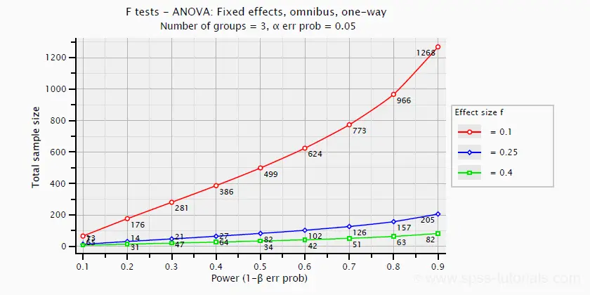
Power and required sample sizes for ANOVA can be computed from Cohen's f and another parameters. The example chart below shows how required sample size relates to power for small, medium and large consequence sizes. Information technology applies to a one-mode ANOVA on iii as large groups.

ANOVA - Omega Squared

A less common just better alternative for (partial) eta-squared is $\omega^two$ or Omega squared computed every bit

$$\omega^2 = \frac{SS_{effect} - df_{effect}\cdot MS_{error}}{SS_{total} + MS_{mistake}}$$

where

$SS$ denotes sums of squares;
$df$ denotes degrees of liberty;
$MS$ denotes mean squares.

Similarly to (partial) eta squared, $\omega^ii$ estimates which proportion of variance in the event variable is accounted for by an event in the unabridged population. The latter, still, is a less biased estimator.^i,2,vi Bones rules of pollex are^five

Small effect: ω ² = 0.01;
Medium effect: ω ² = 0.06;
Large upshot: ω ^two = 0.xiv.

Strangely, $\omega^ii$ is available from JASP only non SPSS. It's also calculated pretty easily by copying a standard ANOVA tabular array into Excel and inbound the formula(south) manually.

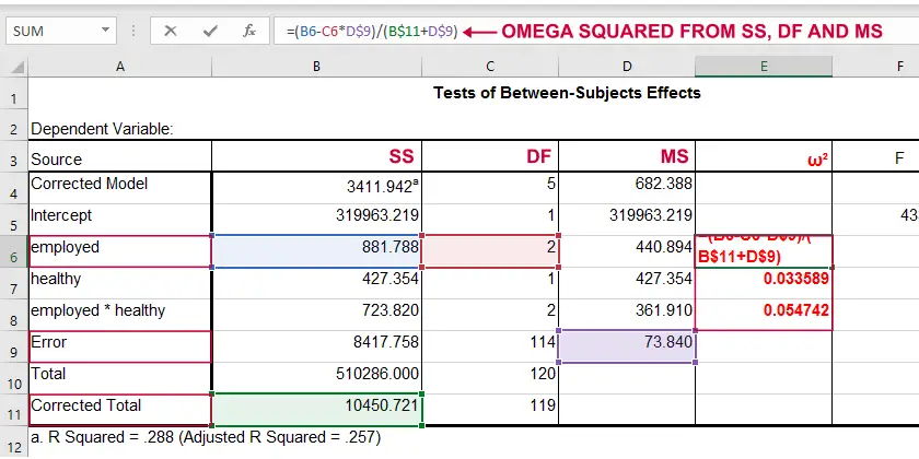Omega Squared Effect Size ANOVA In Excel

Note: you need "Corrected full" for computing omega-squared from SPSS output.

Linear Regression

Effect size measures for (simple and multiple) linear regression are

$\colour{#0a93cd}{f^ii}$ (entire model and private predictor);
$R^ii$ (unabridged model);
$r_{role}^ii$ -squared semipartial (or "part") correlation (private predictor).

Linear Regression - F-Squared

The effect size mensurate of selection for (simple and multiple) linear regression is $f^2$. Bones rules of thumb are that⁸

$f^2$ = 0.02 indicates a modest effect;
$f^2$ = 0.15 indicates a medium issue;
$f^2$ = 0.35 indicates a large effect.

$f^2$ is calculated as

$$f^2 = \frac{R_{inc}^2}{1 - R_{inc}^2}$$

where $R_{inc}^two$ denotes the increase in r-square for a set of predictors over another ready of predictors. Both an entire multiple regression model and an individual predictor are special cases of this general formula.

For an entire model, $R_{inc}^2$ is the r-square increase for the predictors in the model over an empty set of predictors. Without any predictors, we estimate the k hateful of the dependent variable for each observation and we have $R^2 = 0$. In this example, $R_{inc}^two = R^2_{model} - 0 = R^2_{model}$ -the "normal" r-square for a multiple regression model.

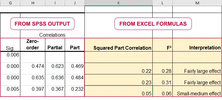
For an individual predictor, $R_{inc}^two$ is the r-square increment resulting from adding this predictor to the other predictor(s) already in the model. It is equal to $r^2_{part}$ -the squared semipartial (or "function") correlation for some predictor. This makes information technology very easy to compute $f^2$ for individual predictors in Excel as shown beneath.

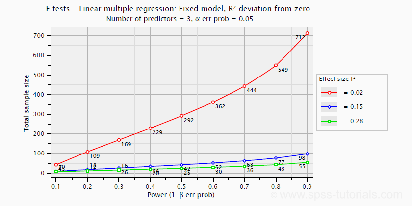
Multiple Regression Effect Size Individual Predictors

$f^2$ is useful for computing the power and/or required sample size for a regression model or individual predictor. Still, these also depend on the number of predictors involved. The effigy below shows how required sample size depends on required ability and estimated (population) effect size for a multiple regression model with 3 predictors.

Linear Regression Power Sample Size Plot

Right, I call back that should do for at present. Nosotros deliberately limited this tutorial to the most important effect size measures in a (peradventure futile) attempt to not overwhelm our readers. If we missed something crucial, please throw the states a comment beneath. Other than that,

thanks for reading!

References

Van den Brink, West.P. & Koele, P. (2002). Statistiek, deel three [Statistics, part 3]. Amsterdam: Nail.
Warner, R.M. (2013). Applied Statistics (2nd. Edition). Thousand Oaks, CA: SAGE.
Agresti, A. & Franklin, C. (2014). Statistics. The Art & Science of Learning from Information. Essex: Pearson Education Limited.
Hair, J.F., Black, W.C., Babin, B.J. et al (2006). Multivariate Data Analysis. New Jersey: Pearson Prentice Hall.
Field, A. (2013). Discovering Statistics with IBM SPSS Statistics. Newbury Park, CA: Sage.
Howell, D.C. (2002). Statistical Methods for Psychology (fifth ed.). Pacific Grove CA: Duxbury.
Siegel, S. & Castellan, N.J. (1989). Nonparametric Statistics for the Behavioral Sciences (2nd ed.). Singapore: McGraw-Hill.
Cohen, J (1988). Statistical Ability Analysis for the Social Sciences (second. Edition). Hillsdale, New Jersey, Lawrence Erlbaum Associates.
Pituch, K.A. & Stevens, J.P. (2016). Applied Multivariate Statistics for the Social Sciences (sixth. Edition). New York: Routledge.